alpenglow.experiments package
Submodules
alpenglow.experiments.AsymmetricFactorExperiment module
-
class
alpenglow.experiments.AsymmetricFactorExperiment.AsymmetricFactorExperiment(dimension=10, begin_min=-0.01, begin_max=0.01, learning_rate=0.05, regularization_rate=0.0, negative_rate=20, cumulative_item_updates=True, norm_type="exponential", gamma=0.8)[source]¶ Bases:
alpenglow.OnlineExperiment.OnlineExperimentImplements the recommendation model introduced in [Paterek2007].
[Paterek2007] Arkadiusz Paterek. „Improving regularized singular value decomposition for collaborative filtering”. In: Proc. KDD Cup Workshop at SIGKDD’07, 13th ACM Int. Conf. on Knowledge Discovery and Data Mining. San Jose, CA, USA, 2007, pp. 39–42. Parameters: - dimension (int) – The latent factor dimension of the factormodel.
- begin_min (double) – The factors are initialized randomly, sampling each element uniformly from the interval (begin_min, begin_max).
- begin_max (double) – See begin_min.
- learning_rate (double) – The learning rate used in the stochastic gradient descent updates.
- regularization_rate (double) – The coefficient for the L2 regularization term.
- negative_rate (int) – The number of negative samples generated after each update. Useful for implicit recommendation.
- norm_type (str) – Type of time decay; either “constant”, “exponential” or “disabled”.
- gamma (double) – Coefficient of time decay in the case of norm_type == “exponential”.
alpenglow.experiments.BatchAndOnlineFactorExperiment module
-
class
alpenglow.experiments.BatchAndOnlineFactorExperiment.BatchAndOnlineFactorExperiment(dimension=10, begin_min=-0.01, begin_max=0.01, batch_learning_rate=0.05, batch_regularization_rate=0.0, batch_negative_rate=70, online_learning_rate=0.05, online_regularization_rate=0.0, online_negative_rate=100)[source]¶ Bases:
alpenglow.OnlineExperiment.OnlineExperimentCombines BatchFactorExperiment and FactorExperiment by updating the model both in batch and continously.
Parameters: - dimension (int) – The latent factor dimension of the factormodel.
- begin_min (double) – The factors are initialized randomly, sampling each element uniformly from the interval (begin_min, begin_max).
- begin_max (double) – See begin_min.
- batch_learning_rate (double) – The learning rate used in the batch stochastic gradient descent updates.
- batch_regularization_rate (double) – The coefficient for the L2 regularization term for batch updates.
- batch_negative_rate (int) – The number of negative samples generated after each batch update. Useful for implicit recommendation.
- timeframe_length (int) – The size of historic time interval to iterate over at every batch model retrain. Leave at the default 0 to retrain on everything.
- online_learning_rate (double) – The learning rate used in the online stochastic gradient descent updates.
- online_regularization_rate (double) – The coefficient for the L2 regularization term for online updata.
- online_negative_rate (int) – The number of negative samples generated after online each update. Useful for implicit recommendation.
alpenglow.experiments.BatchFactorExperiment module
-
class
alpenglow.experiments.BatchFactorExperiment.BatchFactorExperiment(dimension=10, begin_min=-0.01, begin_max=0.01, learning_rate=0.05, regularization_rate=0.0, negative_rate=0.0, number_of_iterations=3, period_length=86400, timeframe_length=0, clear_model=False)[source]¶ Bases:
alpenglow.OnlineExperiment.OnlineExperimentBatch version of
alpenglow.experiments.FactorExperiment.FactorExperiment, meaning it retrains its model periodically nd evaluates the latest model between two training points in an online fashion.Parameters: - dimension (int) – The latent factor dimension of the factormodel.
- begin_min (double) – The factors are initialized randomly, sampling each element uniformly from the interval (begin_min, begin_max).
- begin_max (double) – See begin_min.
- learning_rate (double) – The learning rate used in the stochastic gradient descent updates.
- regularization_rate (double) – The coefficient for the L2 regularization term.
- negative_rate (int) – The number of negative samples generated after each update. Useful for implicit recommendation.
- number_of_iterations (int) – The number of iterations over the data in model retrain.
- period_length (int) – The amount of time between model retrains (seconds).
- timeframe_length (int) – The size of historic time interval to iterate over at every model retrain. Leave at the default 0 to retrain on everything.
- clear_model (bool) – Whether to clear the model between retrains.
alpenglow.experiments.FactorExperiment module
-
class
alpenglow.experiments.FactorExperiment.FactorExperiment(dimension=10, begin_min=-0.01, begin_max=0.01, learning_rate=0.05, regularization_rate=0.0, negative_rate=0.0)[source]¶ Bases:
alpenglow.OnlineExperiment.OnlineExperimentThis class implements an online version of the well-known matrix factorization recommendation model [Koren2009] and trains it via stochastic gradient descent. The model is able to train on implicit data using negative sample generation, see [X.He2016] and the negative_rate parameter.
[Koren2009] Koren, Yehuda, Robert Bell, and Chris Volinsky. “Matrix factorization techniques for recommender systems.” Computer 42.8 (2009). [X.He2016] (1, 2) - He, H. Zhang, M.-Y. Kan, and T.-S. Chua. Fast matrix factorization for online recommendation with implicit feedback. In SIGIR, pages 549–558, 2016.
Parameters: - dimension (int) – The latent factor dimension of the factormodel.
- begin_min (double) – The factors are initialized randomly, sampling each element uniformly from the interval (begin_min, begin_max).
- begin_max (double) – See begin_min.
- learning_rate (double) – The learning rate used in the stochastic gradient descent updates.
- regularization_rate (double) – The coefficient for the L2 regularization term.
- negative_rate (int) – The number of negative samples generated after each update. Useful for implicit recommendation.
alpenglow.experiments.NearestNeighborExperiment module
-
class
alpenglow.experiments.NearestNeighborExperiment.NearestNeighborExperiment(gamma=0.8, norm="num", direction="forward", gamma_thresold=0, num_of_neighbors=10)[source]¶ Bases:
alpenglow.OnlineExperiment.OnlineExperimentThis class implements an online version of a similarity based recommendation model. One of the earliest and most popular collaborative filtering algorithms in practice is the item-based nearest neighbor [Sarwar2001] For these algorithms similarity scores are computed between item pairs based on the co-occurrence of the pairs in the preference of users. Non-stationarity of the data can be accounted for e.g. with the introduction of a time-decay [Ding2005] .
Describing the algorithm more formally, let us denote by
 the set of users that visited item
  , by
, by  the set of items visited by user
  , and by
  the index of item in the sequence of interactions of user . The frequency based time-weighted similarity function is defined by
 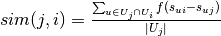 , where
  is the time decaying function. For non-stationary data we sum only over users that visit item
  before item , setting
  if
if  . For stationary data the absolute value of
  is used. The score assigned to item for user is
  The model is represented by the similarity scores. Since computing the model is time consuming, it is done periodically. Moreover, only the most similar items are stored for each item. When the prediction scores are computed for a particular user, all items visited by the user can be considered, including the most recent ones. Hence, the algorithm can be considered semi-online in that it uses the most recent interactions of the current user, but not of the other users. We note that the time decay function is used here to quantify the strength of connection between pairs of items depending on how closely are located in the sequence of a user, and not as a way to forget old data as in [Ding2005].
[Sarwar2001] - Sarwar, G. Karypis, J. Konstan, and J. Reidl. Item-based collaborative filtering recommendation algorithms. In Proc. WWW, pages 285–295, 2001.
[Ding2005] (1, 2) - Ding and X. Li. Time weight collaborative filtering. In Proc. CIKM, pages 485–492. ACM, 2005.
Parameters: - gamma (double) – The constant used in the decay function. It shoud be set to 1 in offline and stationary experiments.
- norm (string) – The type of normalization, can be “num” or “sum”. Defaults to “num” and the other option is not implemented yet.
- direction (string) – It should be set to “both” in offline and stationary experiments.
- gamma_thresold (double) – Threshold to omit very small members when summing similarity. If the value of the decay function is smaller than the threshold, we omit the following members. Defaults to 0 (do not omit small members).
- num_of_neighbors (int) – The number of most similar items that will be stored in the model.
alpenglow.experiments.PersonalPopularityExperiment module
-
class
alpenglow.experiments.PersonalPopularityExperiment.PersonalPopularityExperiment(**parameters)[source]¶ Bases:
alpenglow.OnlineExperiment.OnlineExperimentRecommends the item that the user has watched the most so far; in case of a tie, it falls back to global popularity. Running this model in conjunction with exclude_known == True is not recommended.
alpenglow.experiments.PopularityExperiment module
-
class
alpenglow.experiments.PopularityExperiment.PopularityExperiment(**parameters)[source]¶ Bases:
alpenglow.OnlineExperiment.OnlineExperimentRecommends the most popular item from the set of items seen so far.
alpenglow.experiments.PopularityTimeframeExperiment module
-
class
alpenglow.experiments.PopularityTimeframeExperiment.PopularityTimeframeExperiment(tau=86400)[source]¶ Bases:
alpenglow.OnlineExperiment.OnlineExperimentTime-aware version of PopularityModel, which only considers the last tau time interval when calculating popularities.
Parameters: tau (int) – The time amount to consider.
alpenglow.experiments.SvdppExperiment module
-
class
alpenglow.experiments.SvdppExperiment.SvdppExperiment(begin_min=-0.01, begin_max=0.01, dimension=10, use_sigmoid=False, norm_type="exponential", gamma=0.8, user_vector_weight=0.5, history_weight=0.5)[source]¶ Bases:
alpenglow.OnlineExperiment.OnlineExperimentThis class implements an online version of the SVD++ model [Koren2008] The model is able to train on implicit data using negative sample generation, see [X.He2016] and the negative_rate parameter. We apply a decay on the user history, the weight of the older items is smaller.
[Koren2008] - Koren, “Factorization Meets the Neighborhood: A Multifaceted Collaborative Filtering Model,” Proc. 14th ACM SIGKDD Int’l Conf. Knowledge Discovery and Data Mining, ACM Press, 2008, pp. 426-434.
Parameters: - begin_min (double) – The factors are initialized randomly, sampling each element uniformly from the interval (begin_min, begin_max).
- begin_max (double) – See begin_min.
- dimension (int) – The latent factor dimension of the factormodel.
- learning_rate (double) – The learning rate used in the stochastic gradient descent updates.
- negative_rate (int) – The number of negative samples generated after each update. Useful for implicit recommendation.
- norm_type (string) – Normalization variants.
- gamma (double) – The constant in the decay function.
- user_vector_weight (double) – The user is modeled with a sum of a user vector and a combination of item vectors. The weight of the two part can be set using these parameters.
- history_weight (double) – See user_vector_weight.
alpenglow.experiments.TransitionProbabilityExperiment module
-
class
alpenglow.experiments.TransitionProbabilityExperiment.TransitionProbabilityExperiment(mode_="normal")[source]¶ Bases:
alpenglow.OnlineExperiment.OnlineExperimentA simple algorithm that focuses on the sequence of items a user has visited is one that records how often users visited item i after visiting another item j. This can be viewed as particular form of the item-to-item nearest neighbor with a time decay function that is non-zero only for the immediately preceding item. While the algorithm is more simplistic, it is fast to update the transition fre- quencies after each interaction, thus all recent information is taken into account.
Parameters: mode (string) – The direction of transitions to be considered.