Five minute tutorial
In this tutorial we are going to learn the basic concepts of using Alpenglow by evaluating various baseline models on real world data.
The data
We will use the dataset at http://info.ilab.sztaki.hu/~fbobee/alpenglow/alpenglow_sample_dataset. This is a processed version of the 30M dataset, where we
only keep users above a certain activity threshold
only keep the first events of listening sessions
recode the items so they represent artists instead of tracks
Let’s start by importing standard packages and Alpenglow; and then reading the csv file using pandas. To avoid waiting too much for the experiments to complete, we limit the amount of records read to 200000.
import pandas as pd
import matplotlib
import matplotlib.pyplot as plt
import alpenglow as ag

data = pd.read_csv('http://info.ilab.sztaki.hu/~fbobee/alpenglow/alpenglow_sample_dataset', nrows=200000)
print(data.columns)
Output:
Index(['time', 'user', 'item', 'score', 'eval', 'category'], dtype='object')
To run online experiments, you will need time-series data of user-item interactions in similar format to the above. The only required columns are the ‘user’ and ‘item’ columns – the rest will be autofilled if missing. The most important columns are the following:
time: integer, the timestamp of the record. Controls various things, like evaluation timeframes or batch learning epochs. Defaults to
range(0,len(data))if missing.user: integer, the user the activity belongs to. This column is required.
item: integer, the item the activity belongs to. This column is required.
score: double, the score corresponding to the given record. This could be for example the rating of the item in the case of explicit recommendation. Defaults to constant
1.eval: boolean, whether to run ranking-evaluation on the record. Defaults to constant
True.
Our first model
Let’s start by evaluating a very basic model on the dataset, the popularity model. To do this, we need to import the preconfigured experiment from the package alpenglow.experimens.
from alpenglow.experiments import PopularityExperiment
When creating an instance of the experiment, we can provide various configuration options and parameters.
pop_experiment = PopularityExperiment(
    top_k=100, # we are going to evaluate on top 100 ranking lists
    seed=12345, # for reproducibility, we provide a random seed
)
You can see the list of the available options of online experiments in the documentation of alpenglow.OnlineExperiment and the parameters of this particular experiment in the documentation of the specific implementation (in this case alpenglow.experiments.PopularityExperiment) or, failing that, in the source code of the given class.
Running the experiment on the data is as simple as calling run(data). Multiple options can be provided at this point, for a full list, refer to the documentation of alpenglow.OnlineExperiment.OnlineExperiment.run().
result = pop_experiment.run(data, verbose=True) #this might take a while
The run() method first builds the experiment out of C++ components according to the given parameters, then processes the data, training on it and evaluating the model at the same time. The returned object is a pandas.DataFrame object, which contains various information regarding the results of the experiment:
print(result.columns)
Output:
Index(['time', 'score', 'user', 'item', 'prediction', 'rank'], dtype='object')
Prediction is the score estimate given by the model and rank is the rank of the item in the toplist generated by the model. If the item is not on the toplist, rank is NaN.
The easiest way interpret the results is by using a predefined evaluator, for example alpenglow.evaluation.DcgScore:
from alpenglow.evaluation import DcgScore
result['dcg'] = DcgScore(result)
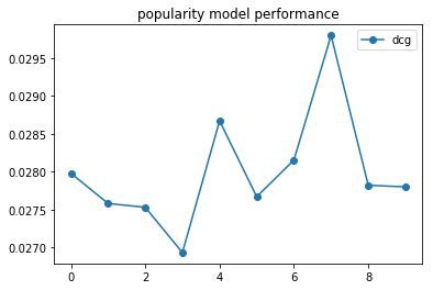
The DcgScore class calculates the NDCG values for the given ranks and returns a pandas.Series object. This can be averaged and plotted easily to visualize the performance of the recommender model.
daily_avg_dcg = result['dcg'].groupby((result['time']-result['time'].min())//86400).mean()
plt.plot(daily_avg_dcg,"o-", label="popularity")
plt.title('popularity model performance')
plt.legend()
Putting it all together:
import pandas as pd
import matplotlib
import matplotlib.pyplot as plt
from alpenglow.evaluation import DcgScore
from alpenglow.experiments import PopularityExperiment

data = pd.read_csv('http://info.ilab.sztaki.hu/~fbobee/alpenglow/alpenglow_sample_dataset', nrows=200000)

pop_experiment = PopularityExperiment(
    top_k=100,
    seed=12345,
)
results = pop_experiment.run(data, verbose=True)
results['dcg'] = DcgScore(results)
daily_avg_dcg = results['dcg'].groupby((results['time']-results['time'].min())//86400).mean()

plt.plot(daily_avg_dcg,"o-", label="popularity")
plt.title('popularity model performance')
plt.legend()
Matrix factorization, hyperparameter search
The alpenglow.experiments.FactorExperiment class implements a factor model, which is updated in an online fashion. After checking the documentation / source, we can see that the most relevant hyperparameters for this model are dimension (the number of latent factors), learning_rate, negative_rate and regularization_rate. For this experiment, we are leaving the factor dimension at the default value of 10, and we don’t need regularization, so we’ll leave it at its default (0) as well. We will find the best negative rate and learning rate using grid search.
We can run the FactorModelExperiment similarly to the popularity model:
from alpenglow.experiments import FactorExperiment
mf_experiment = FactorExperiment(
top_k=100,
)
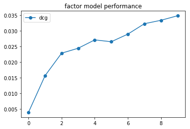
mf_results = mf_experiment.run(data, verbose=True)
mf_results['dcg'] = DcgScore(mf_results)
mf_daily_avg = mf_results['dcg'].groupby((mf_results['time']-mf_results['time'].min())//86400).mean()
plt.plot(mf_daily_avg,"o-", label="factorization")
plt.title('factor model performance')
plt.legend()
The default parameters are chosen to perform generally well. However, the best choice always depends on the task at hand. To find the best values for this particular dataset, we can use Alpenglow’s built in multithreaded hyperparameter search tool: alpenglow.ThreadedParameterSearch.
mf_parameter_search = ag.utils.ThreadedParameterSearch(mf_experiment, DcgScore, threads=4)
mf_parameter_search.set_parameter_values('negative_rate', np.linspace(10, 100, 4))
The ThreadedParameterSearch instance wraps around an OnlineExperiment instance. With each call to the function set_parameter_values, we can set a new dimension for the grid search, which runs the experiments in parallel accoring to the given threads parameter. We can start the hyperparameter search similar to the experiment itself: by calling run().
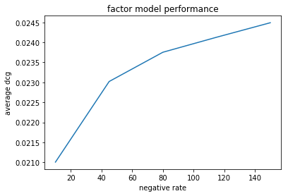
neg_rate_scores = mf_parameter_search.run(data, verbose=False)
The result of the search is a pandas DataFrame, with columns representing the given parameters and the score itself.
plt.plot(neg_rate_scores['negative_rate'], neg_rate_scores['DcgScore'])
plt.ylabel('average dcg')
plt.xlabel('negative rate')
plt.title('factor model performance')